Mastering Geospatial Risk Assessment: A Production-Ready Python Approach

In today’s data-driven landscape, knowing where a risk lies is just as important as knowing what the risk is. Whether for insurance underwriting, urban planning, or disaster response, Geospatial Risk Assessment transforms raw location data into actionable intelligence.
This guide expands on the foundational concepts from Araz Shah's repository, providing a robust, modular framework for calculating risk scores using Python.
1. The Architectural Blueprint
Spaghetti code is the enemy of scalable GIS analysis. A modular directory structure ensures your risk model is maintainable and testable.
Recommended Structure:
geospatial-risk-assessment/
├── src/
│ ├── __init__.py
│ ├── data_loader.py # Ingestion & CRS normalization
│ ├── preprocessor.py # Spatial joins & cleaning
│ ├── risk_engine.py # The math: Hazard * Vulnerability * Exposure
│ └── visualizer.py # Map generation (Folium/Matplotlib)
├── data/
│ ├── raw/ # Original Shapefiles/GeoJSONs
│ └── processed/ # Cleaned parquets
├── notebooks/ # Jupyter notebooks for experimentation
├── config.yaml # Weights and path configurations
└── requirements.txt
2. Robust Data Ingestion
The original example provided a basic loading function. In a real-world scenario, we must handle Coordinate Reference Systems (CRS) strictly. Mixing CRS (e.g., Lat/Lon vs. Projected Meters) is the #1 cause of silent errors in spatial analysis.
Improved Implementation:
import geopandas as gpd
from pathlib import Path
from typing import Optional
import logging

# Configure logging
logging.basicConfig(level=logging.INFO)
logger = logging.getLogger(__name__)

def load_and_normalize_geodata(
    file_path: str,
    target_crs: str = "EPSG:4326"
) -> Optional[gpd.GeoDataFrame]:
    """
    Loads vector data and normalizes the CRS.

    Args:
        file_path: Path to the vector file.
        target_crs: The EPSG code to project data into (default: WGS84).
    """
    path_obj = Path(file_path)

    if not path_obj.exists():
        logger.error(f"File not found: {file_path}")
        return None

    try:
        gdf = gpd.read_file(path_obj)

        # CRS Handling
        if gdf.crs is None:
            logger.warning(f"File {file_path} has no CRS! Assuming {target_crs}, but verify this.")
            gdf.set_crs(target_crs, inplace=True)
        elif gdf.crs.to_string() != target_crs:
            logger.info(f"Reprojecting from {gdf.crs.to_string()} to {target_crs}")
            gdf = gdf.to_crs(target_crs)

        return gdf

    except Exception as e:
        logger.error(f"Failed to load data: {e}")
        return None
3. The Risk Calculation Engine
Risk is rarely a single number; it is a composite of three factors. To calculate it accurately in Python, we must normalize inputs (bring them to a 0-1 scale) so that "Flood Depth (meters)" can be mathematically combined with "Building Cost ($)".
The Formula
$$Risk = (Hazard \\times w\_h) + (Vulnerability \\times w\_v) + (Exposure \\times w\_e)$$
Where $w$ represents the weight assigned to each factor.
Improved Implementation:
import pandas as pd
import numpy as np
from sklearn.preprocessing import MinMaxScaler

class RiskEngine:
    def __init__(self, weights: dict):
        """
        weights: dict, e.g., {'hazard': 0.5, 'vulnerability': 0.3, 'exposure': 0.2}
        """
        self.weights = weights
        self.scaler = MinMaxScaler()

    def normalize_column(self, df: pd.DataFrame, col_name: str) -> pd.Series:
        """Scales a column to a 0-1 range."""
        if col_name not in df.columns:
            raise ValueError(f"Column {col_name} not found.")

        # Reshape for sklearn
        values = df[col_name].values.reshape(-1, 1)
        return self.scaler.fit_transform(values).flatten()

    def calculate_composite_score(
        self,
        gdf: gpd.GeoDataFrame,
        hazard_col: str,
        vuln_col: str,
        exp_col: str
    ) -> gpd.GeoDataFrame:

        working_gdf = gdf.copy()

        # 1. Normalize Inputs
        h_norm = self.normalize_column(working_gdf, hazard_col)
        v_norm = self.normalize_column(working_gdf, vuln_col)
        e_norm = self.normalize_column(working_gdf, exp_col)

        # 2. Apply Weighted Formula
        working_gdf['risk_score'] = (
            (h_norm * self.weights['hazard']) +
            (v_norm * self.weights['vulnerability']) +
            (e_norm * self.weights['exposure'])
        )

        return working_gdf
4. Visualization & Reporting
Once the risk score is calculated, visualization is key for stakeholders. Since you prefer OpenStreetMap (OSM) integration, we can use folium to create interactive heatmaps layered over OSM tiles.
import folium
from folium.plugins import HeatMap

def generate_interactive_map(gdf, output_html="risk_map.html"):
    # Center map on the data centroid
    center_lat = gdf.geometry.centroid.y.mean()
    center_lon = gdf.geometry.centroid.x.mean()

    m = folium.Map(location=[center_lat, center_lon], zoom_start=12, tiles="OpenStreetMap")

    # Add Chloropleth for Risk Score
    folium.Choropleth(
        geo_data=gdf,
        name='Risk Scores',
        data=gdf,
        columns=['id', 'risk_score'],
        key_on='feature.properties.id',
        fill_color='YlOrRd', # Yellow to Red indicates danger
        fill_opacity=0.7,
        line_opacity=0.2,
        legend_name='Composite Risk Score (0-1)'
    ).add_to(m)

    folium.LayerControl().add_to(m)
    m.save(output_html)
    logger.info(f"Map saved to {output_html}")
5. Future Extensions
To take this framework from a script to an enterprise application, consider these next steps:
Spatial Indexing: Implementation of
rtreeor usage of PostGIS as a backend to speed up spatial joins on datasets larger than memory.Raster Integration: Many hazards (floods, fire severity) come as Raster data (GeoTIFF). Implementing
rasterioto sample raster values at vector locations is a critical upgrade.H3 Hexagonal Grid: Instead of using irregular administrative boundaries, aggregate risk into Uber’s H3 hexagonal grid for uniform, comparable spatial units.
Conclusion
By structuring your Python code modularly and rigorously handling coordinate systems and data normalization, you transform simple maps into powerful analytical tools. This approach ensures that your risk assessment is not just a visual exercise, but a reliable metric for decision-making.